Data Preprocessing II

This tutorial contains Python examples for data transformation, focusing on techniques for data normalization and discretization, . Follow the step-by-step instructions below carefully. To execute the code, click on the corresponding cell and press the SHIFT+ENTER keys simultaneously.

Data Transformation I

Sometimes, the original values of an attribute might not be ideally suited for data analysis or modeling purposes. Data transformation is a process that involves converting the entire set of an attribute’s values into a new series of values. The approach is strategically utilized to improve the suitability of the data for different data mining objectives, facilitate more effective analyses, and potentially improve model accuracy and efficiency.

In this tutorial, we’ll focus on the “LotArea” attribute from the house price dataset, exploring transformation functions, data normalization, and data discretization.

Importing Libraries and Configuration

import numpy as np
import pandas as pd
import matplotlib.pyplot as plt
import seaborn as sns
from sklearn import datasets
from sklearn.preprocessing import MinMaxScaler, StandardScaler
from sklearn.cluster import KMeans
from scipy.special import boxcox1p
from scipy.stats import skew
%matplotlib inline
from matplotlib.pylab import rcParams

Settings

# Set the default figure size for matplotlib plots to 15 inches wide by 6 inches tall
rcParams["figure.figsize"] = (15, 6)

# Increase the default font size of the titles in matplotlib plots to extra-extra-large
rcParams["axes.titlesize"] = "xx-large"

# Make the titles of axes in matplotlib plots bold for better visibility
rcParams["axes.titleweight"] = "bold"

# Set the default location of the legend in matplotlib plots to the upper left corner
rcParams["legend.loc"] = "upper left"

# Configure pandas to display all columns of a DataFrame when printed to the console
pd.set_option('display.max_columns', None)

# Configure pandas to display all rows of a DataFrame when printed to the console
pd.set_option('display.max_rows', None)

Load Data

data = datasets.fetch_openml(name="house_prices", as_frame=True)
df = pd.DataFrame(data=data.data, columns=data.feature_names)
df['MedHouseVal'] = data.target
print('Number of samples = %d' % (df.shape[0]))
print('Number of attributes = %d' % (df.shape[1]))
display (df.head(n=10))

Number of samples = 1460
Number of attributes = 81

/opt/conda/lib/python3.11/site-packages/sklearn/datasets/_openml.py:1022: FutureWarning: The default value of `parser` will change from `'liac-arff'` to `'auto'` in 1.4. You can set `parser='auto'` to silence this warning. Therefore, an `ImportError` will be raised from 1.4 if the dataset is dense and pandas is not installed. Note that the pandas parser may return different data types. See the Notes Section in fetch_openml's API doc for details.
  warn(

	Id	MSSubClass	MSZoning	LotFrontage	LotArea	Street	Alley	LotShape	LandContour	Utilities	LotConfig	LandSlope	Neighborhood	Condition1	Condition2	BldgType	HouseStyle	OverallQual	OverallCond	YearBuilt	YearRemodAdd	RoofStyle	RoofMatl	Exterior1st	Exterior2nd	MasVnrType	MasVnrArea	ExterQual	ExterCond	Foundation	BsmtQual	BsmtCond	BsmtExposure	BsmtFinType1	BsmtFinSF1	BsmtFinType2	BsmtFinSF2	BsmtUnfSF	TotalBsmtSF	Heating	HeatingQC	CentralAir	Electrical	1stFlrSF	2ndFlrSF	LowQualFinSF	GrLivArea	BsmtFullBath	BsmtHalfBath	FullBath	HalfBath	BedroomAbvGr	KitchenAbvGr	KitchenQual	TotRmsAbvGrd	Functional	Fireplaces	FireplaceQu	GarageType	GarageYrBlt	GarageFinish	GarageCars	GarageArea	GarageQual	GarageCond	PavedDrive	WoodDeckSF	OpenPorchSF	EnclosedPorch	3SsnPorch	ScreenPorch	PoolArea	PoolQC	Fence	MiscFeature	MiscVal	MoSold	YrSold	SaleType	SaleCondition	MedHouseVal
0	1	60	RL	65.0	8450	Pave	NaN	Reg	Lvl	AllPub	Inside	Gtl	CollgCr	Norm	Norm	1Fam	2Story	7	5	2003	2003	Gable	CompShg	VinylSd	VinylSd	BrkFace	196.0	Gd	TA	PConc	Gd	TA	No	GLQ	706	Unf	0	150	856	GasA	Ex	Y	SBrkr	856	854	0	1710	1	0	2	1	3	1	Gd	8	Typ	0	NaN	Attchd	2003.0	RFn	2	548	TA	TA	Y	0	61	0	0	0	0	NaN	NaN	NaN	0	2	2008	WD	Normal	208500
1	2	20	RL	80.0	9600	Pave	NaN	Reg	Lvl	AllPub	FR2	Gtl	Veenker	Feedr	Norm	1Fam	1Story	6	8	1976	1976	Gable	CompShg	MetalSd	MetalSd	None	0.0	TA	TA	CBlock	Gd	TA	Gd	ALQ	978	Unf	0	284	1262	GasA	Ex	Y	SBrkr	1262	0	0	1262	0	1	2	0	3	1	TA	6	Typ	1	TA	Attchd	1976.0	RFn	2	460	TA	TA	Y	298	0	0	0	0	0	NaN	NaN	NaN	0	5	2007	WD	Normal	181500
2	3	60	RL	68.0	11250	Pave	NaN	IR1	Lvl	AllPub	Inside	Gtl	CollgCr	Norm	Norm	1Fam	2Story	7	5	2001	2002	Gable	CompShg	VinylSd	VinylSd	BrkFace	162.0	Gd	TA	PConc	Gd	TA	Mn	GLQ	486	Unf	0	434	920	GasA	Ex	Y	SBrkr	920	866	0	1786	1	0	2	1	3	1	Gd	6	Typ	1	TA	Attchd	2001.0	RFn	2	608	TA	TA	Y	0	42	0	0	0	0	NaN	NaN	NaN	0	9	2008	WD	Normal	223500
3	4	70	RL	60.0	9550	Pave	NaN	IR1	Lvl	AllPub	Corner	Gtl	Crawfor	Norm	Norm	1Fam	2Story	7	5	1915	1970	Gable	CompShg	Wd Sdng	Wd Shng	None	0.0	TA	TA	BrkTil	TA	Gd	No	ALQ	216	Unf	0	540	756	GasA	Gd	Y	SBrkr	961	756	0	1717	1	0	1	0	3	1	Gd	7	Typ	1	Gd	Detchd	1998.0	Unf	3	642	TA	TA	Y	0	35	272	0	0	0	NaN	NaN	NaN	0	2	2006	WD	Abnorml	140000
4	5	60	RL	84.0	14260	Pave	NaN	IR1	Lvl	AllPub	FR2	Gtl	NoRidge	Norm	Norm	1Fam	2Story	8	5	2000	2000	Gable	CompShg	VinylSd	VinylSd	BrkFace	350.0	Gd	TA	PConc	Gd	TA	Av	GLQ	655	Unf	0	490	1145	GasA	Ex	Y	SBrkr	1145	1053	0	2198	1	0	2	1	4	1	Gd	9	Typ	1	TA	Attchd	2000.0	RFn	3	836	TA	TA	Y	192	84	0	0	0	0	NaN	NaN	NaN	0	12	2008	WD	Normal	250000
5	6	50	RL	85.0	14115	Pave	NaN	IR1	Lvl	AllPub	Inside	Gtl	Mitchel	Norm	Norm	1Fam	1.5Fin	5	5	1993	1995	Gable	CompShg	VinylSd	VinylSd	None	0.0	TA	TA	Wood	Gd	TA	No	GLQ	732	Unf	0	64	796	GasA	Ex	Y	SBrkr	796	566	0	1362	1	0	1	1	1	1	TA	5	Typ	0	NaN	Attchd	1993.0	Unf	2	480	TA	TA	Y	40	30	0	320	0	0	NaN	MnPrv	Shed	700	10	2009	WD	Normal	143000
6	7	20	RL	75.0	10084	Pave	NaN	Reg	Lvl	AllPub	Inside	Gtl	Somerst	Norm	Norm	1Fam	1Story	8	5	2004	2005	Gable	CompShg	VinylSd	VinylSd	Stone	186.0	Gd	TA	PConc	Ex	TA	Av	GLQ	1369	Unf	0	317	1686	GasA	Ex	Y	SBrkr	1694	0	0	1694	1	0	2	0	3	1	Gd	7	Typ	1	Gd	Attchd	2004.0	RFn	2	636	TA	TA	Y	255	57	0	0	0	0	NaN	NaN	NaN	0	8	2007	WD	Normal	307000
7	8	60	RL	NaN	10382	Pave	NaN	IR1	Lvl	AllPub	Corner	Gtl	NWAmes	PosN	Norm	1Fam	2Story	7	6	1973	1973	Gable	CompShg	HdBoard	HdBoard	Stone	240.0	TA	TA	CBlock	Gd	TA	Mn	ALQ	859	BLQ	32	216	1107	GasA	Ex	Y	SBrkr	1107	983	0	2090	1	0	2	1	3	1	TA	7	Typ	2	TA	Attchd	1973.0	RFn	2	484	TA	TA	Y	235	204	228	0	0	0	NaN	NaN	Shed	350	11	2009	WD	Normal	200000
8	9	50	RM	51.0	6120	Pave	NaN	Reg	Lvl	AllPub	Inside	Gtl	OldTown	Artery	Norm	1Fam	1.5Fin	7	5	1931	1950	Gable	CompShg	BrkFace	Wd Shng	None	0.0	TA	TA	BrkTil	TA	TA	No	Unf	0	Unf	0	952	952	GasA	Gd	Y	FuseF	1022	752	0	1774	0	0	2	0	2	2	TA	8	Min1	2	TA	Detchd	1931.0	Unf	2	468	Fa	TA	Y	90	0	205	0	0	0	NaN	NaN	NaN	0	4	2008	WD	Abnorml	129900
9	10	190	RL	50.0	7420	Pave	NaN	Reg	Lvl	AllPub	Corner	Gtl	BrkSide	Artery	Artery	2fmCon	1.5Unf	5	6	1939	1950	Gable	CompShg	MetalSd	MetalSd	None	0.0	TA	TA	BrkTil	TA	TA	No	GLQ	851	Unf	0	140	991	GasA	Ex	Y	SBrkr	1077	0	0	1077	1	0	1	0	2	2	TA	5	Typ	2	TA	Attchd	1939.0	RFn	1	205	Gd	TA	Y	0	4	0	0	0	0	NaN	NaN	NaN	0	1	2008	WD	Normal	118000

Transformation Functions.

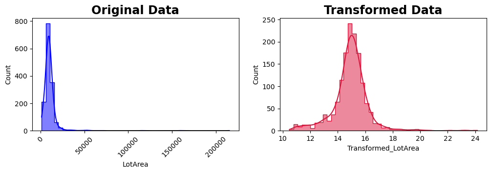
Transformation functions systematically adjust data values. In the following example, we’ll apply a Box-Cox power transformation to the “LotArea” attribute, aiming to reduce skewness and achieve a more symmetric distribution.

skewness_before = skew(df["LotArea"])
print(f"Skewness before transformation: {skewness_before}")

# Apply the Box-Cox transformation (boxcox1p)
lambda_value = 0.1  # A commonly used lambda value for Box-Cox in many scenarios
df["Transformed_LotArea"] = boxcox1p(df["LotArea"], lambda_value)

# Calculate the skewness after transformation
skewness_after = skew(df["Transformed_LotArea"])
print(f"Skewness after transformation: {skewness_after}")

# Plotting the original and transformed data
fig, ax = plt.subplots(1, 2, figsize=(12, 3))

sns.histplot(df["LotArea"], ax=ax[0], kde=True, bins=45, element='step', color='blue')
ax[0].set_title("Original Data")
# rotate x-axis labels
for label in ax[0].get_xticklabels():
    label.set_rotation(45)

sns.histplot(df["Transformed_LotArea"], ax=ax[1], kde=True,  bins=45, element='step', color="crimson")
ax[1].set_title("Transformed Data")

plt.show()

Skewness before transformation: 12.195142125084478
Skewness after transformation: 0.4281475593423937

Data Normalization

Data normalization scales dataset values to a uniform range, crucial for balanced attribute influence in data mining models. The primary methods are:

• Min-max normalization

• Z-score normalization

• Decimal scaling We will demonstrate these techniques on the “LotArea” attribute in the example below.

# Min-Max Normalization
min_max_scaler = MinMaxScaler()
df['Min_Max_Normalized_LotArea'] = min_max_scaler.fit_transform(df[['LotArea']]   )

# Z-Score Normalization (Standardization)
standard_scaler = StandardScaler()
df['Z_Score_Normalized_LotArea'] = standard_scaler.fit_transform(df[['LotArea']]   )

# Decimal Scaling - Manual implementation as before
max_abs_value = df['LotArea'] .abs().max()
num_decimal_places = np.ceil(np.log10(max_abs_value))
df['Decimal_Scaling_Normalized_LotArea'] = df['LotArea']  / (10**num_decimal_places)

# Display the first few rows to verify
display(df[['LotArea', 'Min_Max_Normalized_LotArea', 'Z_Score_Normalized_LotArea', 'Decimal_Scaling_Normalized_LotArea']].head())

	LotArea	Min_Max_Normalized_LotArea	Z_Score_Normalized_LotArea	Decimal_Scaling_Normalized_LotArea
0	8450	0.033420	-0.207142	0.00845
1	9600	0.038795	-0.091886	0.00960
2	11250	0.046507	0.073480	0.01125
3	9550	0.038561	-0.096897	0.00955
4	14260	0.060576	0.375148	0.01426

Data Discretization

Data discretization transforms continuous data into discrete categories or intervals, simplifying the analysis of complex relationships.

• Binning: Grouping data into categories.

• Histogram Analysis: Visualizing data distribution across intervals.

• Clustering Analysis: Organizing data into clusters based on similarity.

We will apply these techniques to the “LotArea” attribute in the upcoming example.

Binning

# Equal-width binning into 4 bins
df['LotArea_Equalwidth'] = pd.cut(df['LotArea'], bins=4, labels=["Small", "Medium", "Large", "Very Large"])
display(df[['LotArea', 'LotArea_Equalwidth']].head())
display(df['LotArea_Equalwidth'].value_counts())

# Equal-depth binning into 4 bins
df['LotArea_EqualDepth'] = pd.qcut(df['LotArea'], q=4, labels=["Small", "Medium", "Large", "Very Large"])
display(df[['LotArea', 'LotArea_EqualDepth']].head())
display(df[ 'LotArea_EqualDepth'].value_counts())

	LotArea	LotArea_Equalwidth
0	8450	Small
1	9600	Small
2	11250	Small
3	9550	Small
4	14260	Small

LotArea_Equalwidth
Small         1453
Medium           3
Large            2
Very Large       2
Name: count, dtype: int64

	LotArea	LotArea_EqualDepth
0	8450	Medium
1	9600	Large
2	11250	Large
3	9550	Large
4	14260	Very Large

LotArea_EqualDepth
Small         365
Medium        365
Large         365
Very Large    365
Name: count, dtype: int64

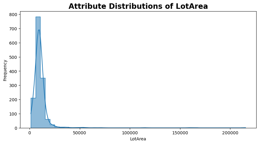
Histogram analysis

plt.figure(figsize=(10, 5))
sns.histplot(df["LotArea"], kde=True, bins=45, element='step', palette='tab10')
plt.title('Attribute Distributions of LotArea')
plt.ylabel('Frequency')
plt.show()

/tmp/ipykernel_3703/3600601536.py:2: UserWarning: Ignoring `palette` because no `hue` variable has been assigned.
  sns.histplot(df["LotArea"], kde=True, bins=45, element='step', palette='tab10')

Clustering analysis

# Apply KMeans clustering
kmeans = KMeans(n_clusters=4, random_state=0).fit(df[['LotArea']])

# Assign cluster labels to each data point for discretization
df['LotArea_Cluster'] = kmeans.labels_

# Optionally, you can map these cluster labels to more meaningful category names
cluster_mapping = {
    0: 'Cluster 1',
    1: 'Cluster 2',
    2: 'Cluster 3',
    3: 'Cluster 4'
}
df['LotArea_Cluster_Label'] = df['LotArea_Cluster'].map(cluster_mapping)

# Display the first few rows to see the clustering-based discretization
display(df[['LotArea', 'LotArea_Cluster', 'LotArea_Cluster_Label']].head())

/opt/conda/lib/python3.11/site-packages/sklearn/cluster/_kmeans.py:1416: FutureWarning: The default value of `n_init` will change from 10 to 'auto' in 1.4. Set the value of `n_init` explicitly to suppress the warning
  super()._check_params_vs_input(X, default_n_init=10)

	LotArea	LotArea_Cluster	LotArea_Cluster_Label
0	8450	0	Cluster 1
1	9600	0	Cluster 1
2	11250	3	Cluster 4
3	9550	0	Cluster 1
4	14260	3	Cluster 4