Introduction to Pandas#
Objective: Develop proficiency in data manipulation and analysis using Pandas, a fundamental Python library renowned for its effectiveness in data science.
This tutorial comprises hands-on examples that guide you through Pandas’ critical features and data handling capabilities. Each example is crafted to illustrate practical approaches to data processing and analysis, enhancing your skill set in real-world applications. To interact with the examples and explore Pandas’ functionalities, select a code cell and press SHIFT-ENTER to execute it.
What is Pandas?#
Pandas is an essential library in Python, renowned for its robust data manipulation and analysis capabilities. Designed primarily for working with structured data, it simplifies handling large datasets and provides intuitive operations for data filtering, aggregation, and visualization. Central to Pandas are its DataFrame and Series data structures, which support a vast array of functions for efficient data manipulation. Whether you’re cleaning, transforming, or analyzing data, Pandas offers the tools needed to make data work more effective and insightful.
Series#
A Series in Pandas is a versatile, one-dimensional array-like structure, capable of holding data of various types. It aligns values and their associated indices, allowing for efficient data retrieval and manipulation. Series objects can be constructed from diverse sources including lists, numpy arrays, or Python dictionaries. The flexibility of a Series extends to its compatibility with numerous numpy functions, thus enabling a broad range of mathematical and statistical operations while maintaining the convenience of index-based data handling inherent to Pandas.
from pandas import Series
import numpy as np

# Creating a Series from a Python list with custom index
temps = Series([22, 23, 19, 25], index=['Mon', 'Tue', 'Wed', 'Thu'])
print(f"Temperatures Series:\n{temps}\n")

# Accessing Series attributes
print(f"Values: {temps.values}")
print(f"Indices: {temps.index}")
print(f"Data type: {temps.dtype}\n")

# Accessing Series elements
print(f"Value at 'Tue': temps['Tue'] = {temps['Tue']}")
print(f"Slice from 'Tue' to 'Thu':temps['Tue':'Thu'] = \n{temps['Tue':'Thu']}")
print(f"Element at position 2 using iloc: temps.iloc[2] = {temps.iloc[2]}")

# Creating a Series from a numpy array
rand_nums = Series(np.random.rand(4))
print(f"\nRandom Numbers Series:\n{rand_nums}\n")

# Creating a Series from a dictionary
fruits_dict = {'apple': 10, 'banana': 20, 'orange': 15}
fruits_series = Series(fruits_dict)
print(f"\nFruits Series:\n{fruits_series}\n")
Temperatures Series:
Mon    22
Tue    23
Wed    19
Thu    25
dtype: int64

Values: [22 23 19 25]
Indices: Index(['Mon', 'Tue', 'Wed', 'Thu'], dtype='object')
Data type: int64

Value at 'Tue': temps['Tue'] = 23
Slice from 'Tue' to 'Thu':temps['Tue':'Thu'] =
Tue    23
Wed    19
Thu    25
dtype: int64
Element at position 2 using iloc: temps.iloc[2] = 19

Random Numbers Series:
0    0.595044
1    0.011953
2    0.295456
3    0.266507
dtype: float64


Fruits Series:
apple     10
banana    20
orange    15
dtype: int64
The following examples cover various aspects of Series in Pandas, including handling of NaN values, boolean filtering, scalar operations, application of numpy functions, and counting discrete values in a Series.#
weather = Series([22, 24, 21, 25, np.nan], index=['Mon', 'Tue', 'Wed', 'Thu', 'Fri'])
print(f"Weather Series:\n{weather}\n")

# Series attributes
print(f"Shape of weather: {weather.shape}")
print(f"Size of weather: {weather.size}")
print(f"Count of non-null elements in weather: {weather.count()}")

# Boolean filtering
print(f"\nDays with temperature above 22:\n{weather[weather > 22]}")

# Scalar operations
print(f"\nIncrementing temperature by 2:\n{weather + 2}")
print(f"Dividing temperature by 2:\n{weather / 2}")

# Applying numpy functions
print(f"\nLog of temperature (adjusted by +1 to handle nan):\n{np.log(weather + 1)}")
print(f"Exponential of temperature:\n{np.exp(weather - 20)}")

# Counting discrete values
moods = Series(["happy", "sad", "neutral", "happy", "sad", np.nan])
print(f"\nMoods Series:\n{moods}\n")
print(f"Count of each mood:\n{moods.value_counts()}")
Weather Series:
Mon    22.0
Tue    24.0
Wed    21.0
Thu    25.0
Fri     NaN
dtype: float64

Shape of weather: (5,)
Size of weather: 5
Count of non-null elements in weather: 4

Days with temperature above 22:
Tue    24.0
Thu    25.0
dtype: float64

Incrementing temperature by 2:
Mon    24.0
Tue    26.0
Wed    23.0
Thu    27.0
Fri     NaN
dtype: float64
Dividing temperature by 2:
Mon    11.0
Tue    12.0
Wed    10.5
Thu    12.5
Fri     NaN
dtype: float64

Log of temperature (adjusted by +1 to handle nan):
Mon    3.135494
Tue    3.218876
Wed    3.091042
Thu    3.258097
Fri         NaN
dtype: float64
Exponential of temperature:
Mon      7.389056
Tue     54.598150
Wed      2.718282
Thu    148.413159
Fri           NaN
dtype: float64

Moods Series:
0      happy
1        sad
2    neutral
3      happy
4        sad
5        NaN
dtype: object

Count of each mood:
happy      2
sad        2
neutral    1
Name: count, dtype: int64
DataFrame#
A DataFrame in Pandas is a tabular, spreadsheet-like data structure where each column can hold data of varying types, including numbers, strings, and booleans. It is more complex than a Series, featuring distinct indices for both rows and columns. DataFrames can be created through various methods, such as from dictionaries, lists of tuples, or arrays from numpy, making them highly versatile for organizing and manipulating different data sets in a table-like format.
# Creating a DataFrame from a dictionary
vehicle_info = {
    "brand": ["Chevrolet", "BMW", "Audi", "Mercedes"],
    "model": ["Camaro", "3 Series", "A4", "C-Class"],
    "price": [35000, 45000, 37000, 50000]
}
vehicle_df = DataFrame(vehicle_info)
print(f"Vehicle Data:\n{vehicle_df}\n")

# Adding new columns to DataFrame
vehicle_df["year"] = 2020
vehicle_df["dealership"] = ["Speed Motors", "Luxury Drives", "Premium Auto", "Elite Cars"]
print(f"Updated Vehicle Data:\n{vehicle_df}\n")

# Creating DataFrame from a list of tuples
sales_data = [
    (2020, 120, 150),
    (2021, 135, 165),
    (2022, 140, 170)
]
sales_columns = ["Year", "Sedan Sales", "SUV Sales"]
sales_df = DataFrame(sales_data, columns=sales_columns)
print(f"Sales Data:\n{sales_df}\n")

# Creating DataFrame from a numpy ndarray
numpy_data = np.random.rand(4, 2)  # create a 4x2 random matrix
numpy_columns = ["Val1", "Val2"]
numpy_df = DataFrame(numpy_data, columns=numpy_columns)
print(f"Numpy DataFrame:\n{numpy_df}\n")

# Accessing DataFrame elements
print(f"Second column of numpy_df:\n{numpy_df['Val2']}\n")
print(f"Type of the second column: {type(numpy_df['Val2'])}\n")

# Accessing a specific DataFrame row
print("Third row of sales data:")
print(sales_df.iloc[2])
print(f"Type of the third row: {type(sales_df.iloc[2])}\n")

# Accessing a specific element
print(f"Specific element (2nd row, 'model' column) in vehicle_df: {vehicle_df.loc[1, 'model']}\n")

# Slicing a DataFrame
print("Slice of vehicle_df (rows 1 to 2, columns 'model' and 'price'):")
print(vehicle_df.iloc[1:3, 1:3])

# Filtering data based on a condition
print(f"Vehicles with price over $40,000:\n{vehicle_df[vehicle_df.price > 40000]}")
---------------------------------------------------------------------------
NameError                                 Traceback (most recent call last)
Cell In[3], line 7
      1 # Creating a DataFrame from a dictionary
      2 vehicle_info = {
      3     "brand": ["Chevrolet", "BMW", "Audi", "Mercedes"],
      4     "model": ["Camaro", "3 Series", "A4", "C-Class"],
      5     "price": [35000, 45000, 37000, 50000]
      6 }
----> 7 vehicle_df = DataFrame(vehicle_info)
      8 print(f"Vehicle Data:\n{vehicle_df}\n")
     10 # Adding new columns to DataFrame

NameError: name 'DataFrame' is not defined
Arithmetic Operations#
# Creating a new DataFrame
np_array1 = np.random.rand(4, 3)
columns = ["A", "B", "C"]
df1 = DataFrame(np_array1, columns=columns)
print(f"DataFrame df1:\n{df1}\n")

# Transposing the DataFrame
print(f"Transposed DataFrame df1:\n{df1.T}\n")

# Arithmetic Operations
print(f"Addition: df1 + 3:\n{df1 + 3}\n")
print(f"Multiplication: df1 * 5:\n{df1 * 5}\n")

# Creating another DataFrame for operation
np_array2 = np.random.rand(4, 3)
df2 = DataFrame(np_array2, columns=columns)
print(f"DataFrame df2:\n{df2}\n")

# Element-wise addition and multiplication
print(f"Element-wise addition: df1 + df2:\n{df1.add(df2)}\n")
print(f"Element-wise multiplication: df1 * df2:\n{df1.mul(df2)}\n")

# Applying functions
print(f"Absolute values in df1:\n{df1.abs()}\n")
print(f"Maximum value in each column of df1:\n{df1.max()}\n")
print(f"Minimum value in each row of df1:\n{df1.min(axis=1)}\n")
print(f"Sum of each column in df1:\n{df1.sum()}\n")
print(f"Average of each row in df1:\n{df1.mean(axis=1)}\n")

# Custom function application
max_min_diff = lambda x: x.max() - x.min()
print(f"Max - Min per column in df1:\n{df1.apply(max_min_diff)}\n")
print(f"Max - Min per row in df1:\n{df1.apply(max_min_diff, axis=1)}\n")

# Applying value_counts to DataFrame
shape_colors = DataFrame({
    "shape": ["triangle", "circle", "circle", "square", "triangle", "square"],
    "color": ["green", "green", "red", "red", "blue", "blue"]
})
print(f"Shapes and Colors DataFrame:\n{shape_colors}\n")
print(f"Counts of unique shape and color combinations:\n{shape_colors.value_counts().sort_index()}")
DataFrame df1:
          A         B         C
0  0.018381  0.055265  0.347357
1  0.656001  0.139697  0.339375
2  0.742442  0.681375  0.801696
3  0.631857  0.251695  0.409332

Transposed DataFrame df1:
          0         1         2         3
A  0.018381  0.656001  0.742442  0.631857
B  0.055265  0.139697  0.681375  0.251695
C  0.347357  0.339375  0.801696  0.409332

Addition: df1 + 3:
          A         B         C
0  3.018381  3.055265  3.347357
1  3.656001  3.139697  3.339375
2  3.742442  3.681375  3.801696
3  3.631857  3.251695  3.409332

Multiplication: df1 * 5:
          A         B         C
0  0.091904  0.276325  1.736783
1  3.280004  0.698487  1.696873
2  3.712210  3.406876  4.008478
3  3.159287  1.258475  2.046659

DataFrame df2:
          A         B         C
0  0.652178  0.350798  0.661221
1  0.257208  0.758696  0.361774
2  0.036578  0.760356  0.585513
3  0.446599  0.258286  0.475202

Element-wise addition: df1 + df2:
          A         B         C
0  0.670559  0.406063  1.008578
1  0.913209  0.898393  0.701148
2  0.779020  1.441731  1.387208
3  1.078456  0.509981  0.884534

Element-wise multiplication: df1 * df2:
          A         B         C
0  0.011988  0.019387  0.229680
1  0.168728  0.105988  0.122777
2  0.027157  0.518088  0.469403
3  0.282187  0.065009  0.194515

Absolute values in df1:
          A         B         C
0  0.018381  0.055265  0.347357
1  0.656001  0.139697  0.339375
2  0.742442  0.681375  0.801696
3  0.631857  0.251695  0.409332

Maximum value in each column of df1:
A    0.742442
B    0.681375
C    0.801696
dtype: float64

Minimum value in each row of df1:
0    0.018381
1    0.139697
2    0.681375
3    0.251695
dtype: float64

Sum of each column in df1:
A    2.048681
B    1.128033
C    1.897759
dtype: float64

Average of each row in df1:
0    0.140334
1    0.378358
2    0.741838
3    0.430961
dtype: float64

Max - Min per column in df1:
A    0.724061
B    0.626110
C    0.462321
dtype: float64

Max - Min per row in df1:
0    0.328976
1    0.516303
2    0.120320
3    0.380162
dtype: float64

Shapes and Colors DataFrame:
      shape  color
0  triangle  green
1    circle  green
2    circle    red
3    square    red
4  triangle   blue
5    square   blue

Counts of unique shape and color combinations:
shape     color
circle    green    1
          red      1
square    blue     1
          red      1
triangle  blue     1
          green    1
dtype: int64
Plotting Series and DataFrame#
import pandas as pd
import matplotlib.pyplot as plt
%matplotlib inline
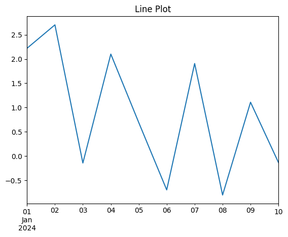
# Line Plot
s = Series(np.random.randn(10), index=pd.date_range('1/1/2024', periods=10))
s.plot(kind='line', title='Line Plot')
plt.show()
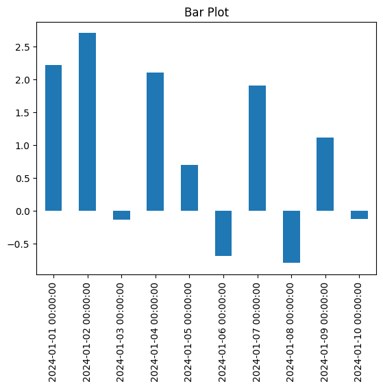
# Bar Plot
s.plot(kind='bar', title='Bar Plot')
plt.show()
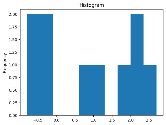
# Histogram
s.plot(kind='hist', title='Histogram')
plt.show()
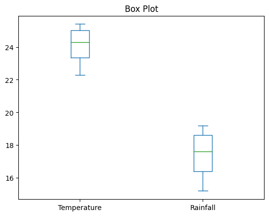
# Box Plot
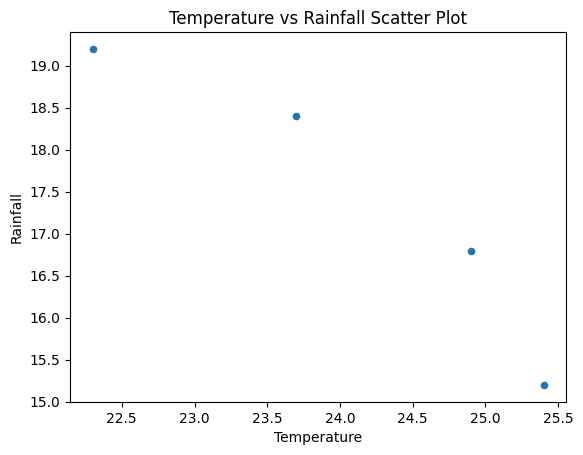
data_tuples = [
(2020, 25.4, 15.2),
(2021, 24.9, 16.8),
(2022, 23.7, 18.4),
(2023, 22.3, 19.2)
]
columns = ["Year", "Temperature", "Rainfall"]
weather_df = DataFrame(data_tuples, columns=columns)
weather_df[['Temperature', 'Rainfall']].plot(kind='box', title='Box Plot')
plt.show()
# Scatter Plot
weather_df.plot(kind='scatter', x='Temperature', y='Rainfall', title='Temperature vs Rainfall Scatter Plot')
plt.show()